Tutorial Distance-Based Selectors#
This tutorial demonstrates using distance-based selectors in selector package. To easily visualize the data and sampled points, we will use a 2D dataset in this tutorial. However, the same functionality can be applied to higher dimensional datasets.
import sys

# uncomment the following line to run the code for your own project directory
# sys.path.append("/Users/Someone/Documents/projects/Selector")
import matplotlib.pylab as plt
import numpy as np
from sklearn.datasets import make_blobs
from sklearn.metrics.pairwise import pairwise_distances
from IPython.display import Markdown

from selector.methods.distance import MaxMin, MaxSum, OptiSim, DISE
from selector.measures.diversity import compute_diversity
Utility Function for Plotting Data#
# define a function to make visualization easier


def graph_data(
    data,
    indices=None,
    labels=None,
    reference=False,
    title="",
    xlabel="",
    ylabel="",
    number=False,
    fname=None,
):
    """Graphs the data in a scatter plot.

    Parameters
    ----------
    data : numpy.ndarray of shape (n_samples, 2)
        The original data points to be graphed.
    indices : list of numpy.ndarray, optional
        List of indices array of the data points selected.
    labels : list of str, optional
        List of labels denoting method for selected indices.
    reference : bool, optional
        Whether to highlight the first data point.
    title : str, optional
        The title of the plot.
    xlabel : str, optional
        The label of the x-axis.
    ylabel : str, optional
        The label of the y-axis.
    number : bool, optional
        Whether to label the selected data points with numbers representing the order of selection.
    fname : str, optional
        Filename for saving the figure. If None, figure is shown.

    """
    if data.ndim != 2 or data.shape[1] != 2:
        raise ValueError(f"Expect data to be a 2D array with 2 columns, got {data.shape}.")

    if labels is not None and len(indices) != len(labels):
        raise ValueError(
            f"Expect indices and labels to have the same length, got {len(indices)} and {len(labels)}."
        )

    # Add a title and axis labels
    plt.figure(dpi=100)
    plt.title(title, fontsize=18)
    plt.xlabel(xlabel, fontsize=14)
    plt.ylabel(ylabel, fontsize=14)

    # plot original data
    plt.scatter(data[:, 0], data[:, 1], marker="o", facecolors="none", edgecolors="0.75")

    colors = ["skyblue", "r", "b", "k", "g", "orange", "navy", "indigo", "pink", "purple", "yellow"]
    markers = ["o", "x", "*", "_", "|", "s", "p", ">", "<", "^", "v"]
    text_location = [(0.1, 0.1), (-0.1, 0.1)]
    colors_numbers = ["black", "red", "blue", "k", "k", "k", "k", "k", "k", "k", "k"]

    if indices:
        for index, selected_index in enumerate(indices):
            plt.scatter(
                data[selected_index, 0],
                data[selected_index, 1],
                c=colors[index],
                label=labels[index] if labels is not None else None,
                marker=markers[index],
            )
            if number:
                shift_x, shift_y = text_location[index]
                for i, mol_id in enumerate(selected_index):
                    plt.text(
                        data[mol_id, 0] + shift_x,
                        data[mol_id, 1] + shift_y,
                        str(i + 1),
                        c=colors_numbers[index],
                    )
    if reference:
        plt.scatter(data[0, 0], data[0, 1], c="black")
    if labels is not None:
        # plt.legend(loc="upper left", frameon=False)
        plt.legend(loc="best", frameon=True)
    if fname is not None:
        plt.savefig(fname, dpi=500)
    else:
        plt.show()
# define function to render tables easier


def render_table(data, caption=None, decimals=3):
    """Renders a list of lists in ta markdown table for easy visualization.

    Parameters
    ----------
    data : list of lists
        The data to be rendered in a table, each inner list represents a row with the first row
        being the header.
    caption : str, optional
        The caption of the table.
    decimals : int, optional
        The number of decimal places to round the data to.
    """

    # check all rows have the same number of columns
    if not all(len(row) == len(data[0]) for row in data):
        raise ValueError("Expect all rows to have the same number of columns.")

    if caption is not None:
        # check if caption is a string
        if not isinstance(caption, str):
            raise ValueError("Expect caption to be a string.")
        tmp_output = f"**{caption}**\n\n"

    # get the width of each column (transpose the data list and get the max length of each new row)
    colwidths = [max(len(str(s)) for s in col) + 2 for col in zip(*data)]

    # construct the header row
    header = f"| {' | '.join(f'{str(s):^{w}}' for s, w in zip(data[0], colwidths))} |"
    tmp_output += header + "\n"

    # construct a separator row
    separator = f"|{'|'.join(['-' * w for w in colwidths])}|"
    tmp_output += separator + "\n"

    # construct the data rows
    for row in data[1:]:
        # round the data to the specified number of decimal places
        row = [round(s, decimals) if isinstance(s, float) else s for s in row]
        row_str = f"| {' | '.join(f'{str(s):^{w}}' for s, w in zip(row, colwidths))} |"
        tmp_output += row_str + "\n"

    return display(Markdown(tmp_output))
Generating Data#
The data should be provided as:
either an array
Xof shape(n_samples, n_features)encodingn_samplessamples (rows) each inn_features-dimensional (columns) feature space,or an array
X_distof shape(n_samples, n_samples)encoding the distance (i.e., dissimilarity) between each pair ofn_samplessample points.
This data can be loaded from various file formats (e.g., csv, npz, txt, etc.) or generated using various libraries on the fly. In this tutorial, we use sklearn.datasets.make_blobs to generate cluster(s) of n_samples points in 2-dimensions (n-features=2), so that it can be easily visualized. However, the same functionality can be applied to higher dimensional datasets.
Selecting from One Cluster#
# generate n_sample data in 2D feature space forming 1 cluster
X, labels = make_blobs(
    n_samples=500,
    n_features=2,
    centers=np.array([[0.0, 0.0]]),
    random_state=42,
)

# compute the (n_sample, n_sample) pairwise distance matrix
X_dist = pairwise_distances(X, metric="euclidean")

print("Shape of data   = ", X.shape)
print("Shape of labels = ", labels.shape)
print("Unique labels   = ", np.unique(labels))
print("Cluster size    = ", np.count_nonzero(labels == 0))
print("Shape of the distance array = ", X_dist.shape)
Shape of data   =  (500, 2)
Shape of labels =  (500,)
Unique labels   =  [0]
Cluster size    =  500
Shape of the distance array =  (500, 500)
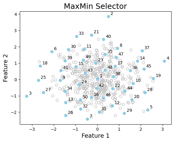
Example 1: MaxMin Selector#
The MaxMin method selects the subset that maximizes the minimum distance to all previously selected points. This method requires the pairwise distance between all points in the dataset, so it is not recommended for large datasets. To select subsets of points, either the dataset’s pairwise distance matrix X_dist or the feature matrix X should be provided. The latter requires specification of fun_dist(X) -> X_dist function for computing the pairwise distance between points. This can be a user-defined function or a sklearn.metrics.pairwise_distances function, as shown below. Check MaxMin Documentation for more details.
# select samples using X_dist
collector = MaxMin()
indices_1 = collector.select(X_dist, size=50)

# select samples using X given a distance function (to compute the distance matrix)
collector = MaxMin(fun_dist=lambda x: pairwise_distances(x, metric="euclidean"))
indices_2 = collector.select(X, size=50)

# check if the selected samples are the same
assert indices_1 == indices_2

# visualize data and selected samples (in the order selected)
graph_data(
    X,
    indices=[indices_1],
    labels=None,
    title="MaxMin Selector",
    xlabel="Feature 1",
    ylabel="Feature 2",
    number=True,
)
Example 2: Directed Sphere Exclusion (DISE) Selector#
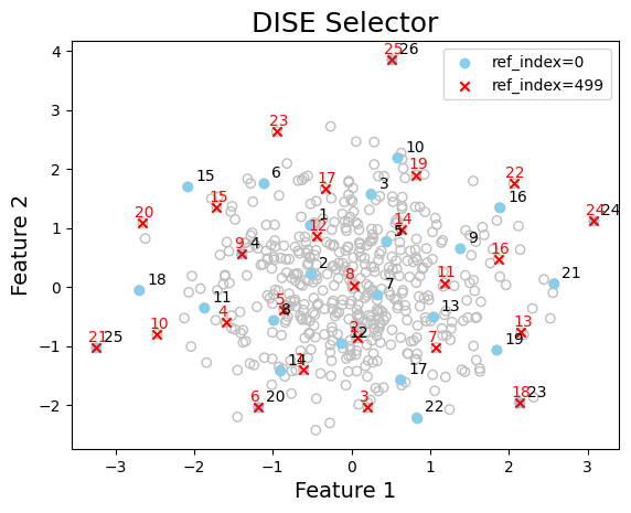
This selector can be used in a similar fashion, however, there are user-defined parameters that can influence the selected subset.
For example, ref_index specifies the index of the reference point which is the first point sampled, and p denotes which Minkowski p-norm to use for computing the distance between points. The default value of p=2 corresponds to the Euclidean distance. Check DISE Documentation for more details.
collector = DISE(ref_index=0, p=2)
indices_1 = collector.select(X_dist, size=25)

collector = DISE(ref_index=499, p=2)
indices_2 = collector.select(X_dist, size=25)

# visualize data and selected samples (in the order selected)
graph_data(
    X,
    indices=[indices_1, indices_2],
    labels=["ref_index=0", "ref_index=499"],
    title="DISE Selector",
    xlabel="Feature 1",
    ylabel="Feature 2",
    number=True,
)
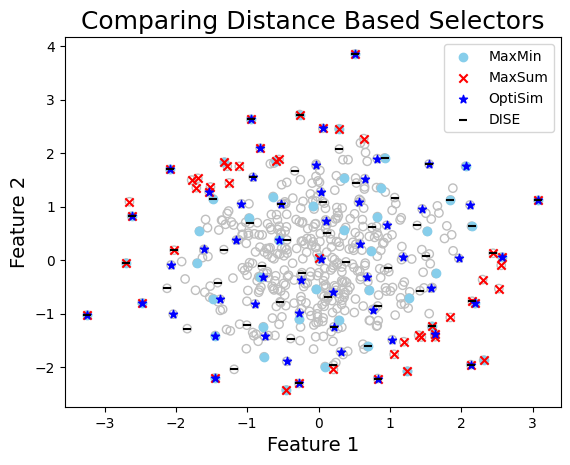
Comparing Multiple Selection Methods (One Cluster)#
Distance-Based Methods#
Check Documentation: MaxMin | MaxSum | OptiSim | DISE
from scipy.spatial.distance import pdist, squareform

# select data using distance base methods
# ---------------------------------------
size = 50

collector = MaxMin()
index_maxmin = collector.select(X_dist, size=size)

collector = MaxSum(fun_dist=lambda x: squareform(pdist(x, metric="minkowski", p=0.1)))
index_maxsum = collector.select(X, size=size)

collector = OptiSim(ref_index=0, tol=0.1)
index_optisim = collector.select(X_dist, size=size)

collector = DISE(ref_index=0, p=2.0)
index_dise = collector.select(X, size=size)

graph_data(
    X,
    indices=[index_maxmin, index_maxsum, index_optisim, index_dise],
    labels=["MaxMin", "MaxSum", "OptiSim", "DISE"],
    title="Comparing Distance Based Selectors",
    xlabel="Feature 1",
    ylabel="Feature 2",
    fname="quick_start_compare_distance_methods",
)
Compute diversity of selected points#
The diversity of a set of points can be computed using the compute_diversity using any of the several diversity metrics provided in qc_selector.diversity module. Here the log determinant function (logdet) and the Wasserstein Distance to Uniform Distribution (wdud) are used to compute the diversity of the selected points. Higher logdet and lower wdud values indicate higher diversity of the selected points.
div_measure = ["logdet", "wdud"]
seleced_sets = zip(
    ["MaxMin", "MaxSum", "OptiSim", "DISE"],
    [index_maxmin, index_maxsum, index_optisim, index_dise],
)

# compute the diversity of the selected sets and render the results in a table
table_data = [[""] + div_measure]
for i in seleced_sets:
    # print([i[0]] + [compute_diversity(X[i[1]], div_type=m) for m in div_measure])
    table_data.append([i[0]] + [compute_diversity(X_dist[i[1]], div_type=m) for m in div_measure])

render_table(table_data, caption="Diversity of Selected Sets")
Diversity of Selected Sets
| | logdet | wdud | |———|——————-|———————| | MaxMin | 94.308 | 0.068 | | MaxSum | 72.739 | 0.09 | | OptiSim | 97.782 | 0.076 | | DISE | 94.848 | 0.077 |
Comparing Multiple Selection Methods (Multiple Clusters)#
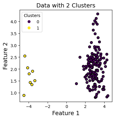
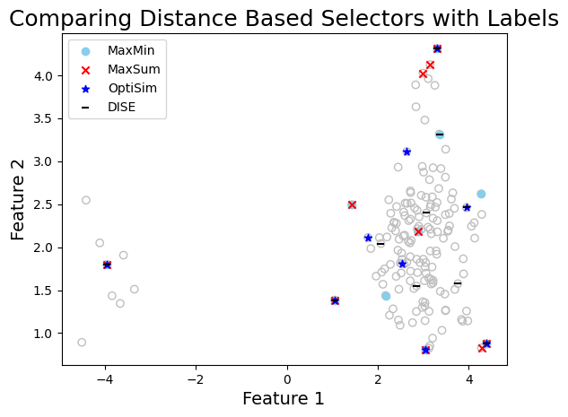
Each cluster is treated independently, and if possible, equal number of samples are selected from each cluster. However, if a cluster is underpopulated, then all points from that cluster are selected. This is to ensure that the selected subset is representative of the entire dataset.
# generate n_sample data in 2D feature space forming 3 clusters
# X, labels = make_blobs(n_samples=500, n_features=2, centers=2, random_state=42)

X, labels = make_blobs(
    n_samples=[150, 5, 8],  # cluster sizes
    centers=[(3, 2), (3, 4), (-4, 1.5)],  # fixed centers for clear separation
    n_features=2,
    cluster_std=[0.6, 0.2, 0.5],  # per-cluster spread
    random_state=42,
)
# update labels as we intentially merged two clusters
labels[labels == 1] = 0
labels[labels == 2] = 1

# plot the coordinates with the updated labels
plt.figure(figsize=(4, 4))
plt.title("Data with 2 Clusters", fontsize=14)
plt.xlabel("Feature 1", fontsize=14)
plt.ylabel("Feature 2", fontsize=14)
scatter = plt.scatter(X[:, 0], X[:, 1], c=labels, cmap="viridis", marker="o", edgecolors="k")
plt.legend(*scatter.legend_elements(), title="Clusters")
plt.show()
# compute the (n_sample, n_sample) pairwise distance matrix
X_dist = pairwise_distances(X, metric="euclidean")

print("Shape of data   = ", X.shape)
print("Shape of labels = ", labels.shape)
print("Unique labels   = ", np.unique(labels))
size_0, size_1 = np.count_nonzero(labels == 0), np.count_nonzero(labels == 1)
print("Cluster sizes = ", size_0, size_1)
print("Shape of the distance array = ", X_dist.shape)
Shape of data   =  (163, 2)
Shape of labels =  (163,)
Unique labels   =  [0 1]
Cluster sizes =  155 8
Shape of the distance array =  (163, 163)
To select from multiple clusters provide the labels argument to the select method.
Check Documentation: MaxMin | MaxSum | OptiSim | DISE
# select data using distance base methods with labels
# ---------------------------------------------------
size = 10

collector = MaxMin()
index_maxmin = collector.select(X_dist, size=size, labels=labels)

collector = MaxSum()
index_maxsum = collector.select(X_dist, size=size, labels=labels)

collector = OptiSim(ref_index=0, tol=0.1)
index_optisim = collector.select(X_dist, size=size, labels=labels)

collector = DISE(ref_index=0, p=2.0)
index_dise = collector.select(X, size=size, labels=labels)

graph_data(
    X,
    indices=[index_maxmin, index_maxsum, index_optisim, index_dise],
    labels=["MaxMin", "MaxSum", "OptiSim", "DISE"],
    title="Comparing Distance Based Selectors with Labels",
    xlabel="Feature 1",
    ylabel="Feature 2",
)
div_measure = ["logdet", "wdud"]
seleced_sets = zip(
    ["MaxMin", "MaxSum", "OptiSim", "DISE"],
    [index_maxmin, index_maxsum, index_optisim, index_dise],
)

# compute the diversity of the selected sets and render the results in a table
table_data = [[""] + div_measure]
for i in seleced_sets:
    # print([i[0]] + [compute_diversity(X[i[1]], div_type=m) for m in div_measure])
    table_data.append([i[0]] + [compute_diversity(X_dist[i[1]], div_type=m) for m in div_measure])

render_table(table_data, caption="Diversity of Selected Sets")
Diversity of Selected Sets
| | logdet | wdud | |———|——————–|———————| | MaxMin | 36.484 | 0.247 | | MaxSum | 33.63 | 0.233 | | OptiSim | 35.184 | 0.249 | | DISE | 35.998 | 0.259 |
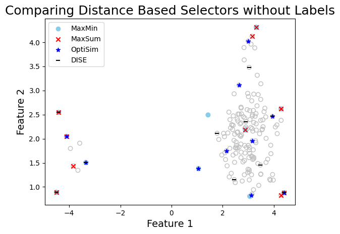
To better demonstrate how the labels can facilitate selection from multiple clusters, let’s check
what if we don’t provide the labels argument to the select method. In this case, the selection methods will treat the entire dataset as one cluster and select points accordingly. This may lead to underrepresentation of some clusters in the selected subset, especially if the clusters are of varying densities or sizes.
# select data using distance base methods with labels
# ---------------------------------------------------
size = 10

collector = MaxMin()
index_maxmin = collector.select(X_dist, size=size, labels=None)

collector = MaxSum()
index_maxsum = collector.select(X_dist, size=size, labels=None)

collector = OptiSim(ref_index=0, tol=0.1)
index_optisim = collector.select(X_dist, size=size, labels=None)

collector = DISE(ref_index=0, p=2.0)
index_dise = collector.select(X, size=size, labels=None)

graph_data(
    X,
    indices=[index_maxmin, index_maxsum, index_optisim, index_dise],
    labels=["MaxMin", "MaxSum", "OptiSim", "DISE"],
    title="Comparing Distance Based Selectors without Labels",
    xlabel="Feature 1",
    ylabel="Feature 2",
)
div_measure = ["logdet", "wdud"]
seleced_sets = zip(
    ["MaxMin", "MaxSum", "OptiSim", "DISE"],
    [index_maxmin, index_maxsum, index_optisim, index_dise],
)

# compute the diversity of the selected sets and render the results in a table
table_data = [[""] + div_measure]
for i in seleced_sets:
    # print([i[0]] + [compute_diversity(X[i[1]], div_type=m) for m in div_measure])
    table_data.append([i[0]] + [compute_diversity(X_dist[i[1]], div_type=m) for m in div_measure])

render_table(table_data, caption="Diversity of Selected Sets")
Diversity of Selected Sets
| | logdet | wdud | |———|——————–|———————| | MaxMin | 37.537 | 0.154 | | MaxSum | 32.678 | 0.145 | | OptiSim | 36.661 | 0.2 | | DISE | 36.818 | 0.181 |

