Tutorial Partition-Based Selectors#
This tutorial demonstrates using partition-based selectors in selector package. To easily visualize the data and sampled points, we will use a 2D dataset in this tutorial. However, the same functionality can be applied to higher dimensional datasets.
import sys

# uncomment the following line to run the code for your own project directory
# sys.path.append("/Users/Someone/Documents/projects/Selector")
import matplotlib.pylab as plt
import numpy as np
from sklearn.datasets import make_blobs
from sklearn.metrics.pairwise import pairwise_distances
from IPython.display import Markdown

from selector.measures.diversity import compute_diversity
from selector.methods.partition import Medoid, GridPartition
Utility Function for Plotting Data#
# define a function to make visualization easier


def graph_data(
    data,
    indices=None,
    labels=None,
    reference=False,
    title="",
    xlabel="",
    ylabel="",
    number=False,
    fname=None,
):
    """Graphs the data in a scatter plot.

    Parameters
    ----------
    data : numpy.ndarray of shape (n_samples, 2)
        The original data points to be graphed.
    indices : list of numpy.ndarray, optional
        List of indices array of the data points selected.
    labels : list of str, optional
        List of labels denoting method for selected indices.
    reference : bool, optional
        Whether to highlight the first data point.
    title : str, optional
        The title of the plot.
    xlabel : str, optional
        The label of the x-axis.
    ylabel : str, optional
        The label of the y-axis.
    number : bool, optional
        Whether to label the selected data points with numbers representing the order of selection.
    fname : str, optional
        Filename for saving the figure. If None, figure is shown.
    """
    if data.ndim != 2 or data.shape[1] != 2:
        raise ValueError(f"Expect data to be a 2D array with 2 columns, got {data.shape}.")

    if labels is not None and len(indices) != len(labels):
        raise ValueError(
            f"Expect indices and labels to have the same length, got {len(indices)} and {len(labels)}."
        )

    # Add a title and axis labels
    plt.figure(dpi=100)
    plt.title(title, fontsize=18)
    plt.xlabel(xlabel, fontsize=14)
    plt.ylabel(ylabel, fontsize=14)

    # plot original data
    plt.scatter(data[:, 0], data[:, 1], marker="o", facecolors="none", edgecolors="0.75")

    colors = ["skyblue", "r", "b", "k", "g", "orange", "navy", "indigo", "pink", "purple", "yellow"]
    markers = ["o", "x", "*", "_", "|", "s", "p", ">", "<", "^", "v"]
    text_location = [(0.1, 0.1), (-0.1, 0.1)]
    colors_numbers = ["black", "red", "blue", "k", "k", "k", "k", "k", "k", "k", "k"]

    if indices:
        for index, selected_index in enumerate(indices):
            plt.scatter(
                data[selected_index, 0],
                data[selected_index, 1],
                c=colors[index],
                label=labels[index] if labels is not None else None,
                marker=markers[index],
            )
            if number:
                shift_x, shift_y = text_location[index]
                for i, mol_id in enumerate(selected_index):
                    plt.text(
                        data[mol_id, 0] + shift_x,
                        data[mol_id, 1] + shift_y,
                        str(i + 1),
                        c=colors_numbers[index],
                    )
    if reference:
        plt.scatter(data[0, 0], data[0, 1], c="black")
    if labels is not None:
        # plt.legend(loc="upper left", frameon=False)
        plt.legend(loc="best", frameon=False)
    if fname is not None:
        plt.savefig(fname, dpi=500)
    else:
        plt.show()
# define function to render tables easier


def render_table(data, caption=None, decimals=3):
    """Renders a list of lists in ta markdown table for easy visualization.

    Parameters
    ----------
    data : list of lists
        The data to be rendered in a table, each inner list represents a row with the first row
        being the header.
    caption : str, optional
        The caption of the table.
    decimals : int, optional
        The number of decimal places to round the data to.
    """

    # check all rows have the same number of columns
    if not all(len(row) == len(data[0]) for row in data):
        raise ValueError("Expect all rows to have the same number of columns.")

    if caption is not None:
        # check if caption is a string
        if not isinstance(caption, str):
            raise ValueError("Expect caption to be a string.")
        tmp_output = f"**{caption}**\n\n"

    # get the width of each column (transpose the data list and get the max length of each new row)
    colwidths = [max(len(str(s)) for s in col) + 2 for col in zip(*data)]

    # construct the header row
    header = f"| {' | '.join(f'{str(s):^{w}}' for s, w in zip(data[0], colwidths))} |"
    tmp_output += header + "\n"

    # construct a separator row
    separator = f"|{'|'.join(['-' * w for w in colwidths])}|"
    tmp_output += separator + "\n"

    # construct the data rows
    for row in data[1:]:
        # round the data to the specified number of decimal places
        row = [round(s, decimals) if isinstance(s, float) else s for s in row]
        row_str = f"| {' | '.join(f'{str(s):^{w}}' for s, w in zip(row, colwidths))} |"
        tmp_output += row_str + "\n"

    return display(Markdown(tmp_output))
Generating Data#
The data should be provided as:
either an array
Xof shape(n_samples, n_features)encodingn_samplessamples (rows) each inn_features-dimensional (columns) feature space,or an array
X_distof shape(n_samples, n_samples)encoding the distance (i.e., dissimilarity) between each pair ofn_samplessample points.
This data can be loaded from various file formats (e.g., csv, npz, txt, etc.) or generated using various libraries on the fly. In this tutorial, we use sklearn.datasets.make_blobs to generate cluster(s) of n_samples points in 2-dimensions (n-features=2), so that it can be easily visualized. However, the same functionality can be applied to higher dimensional datasets.
Selecting from One Cluster#
# generate n_sample data in 2D feature space forming 1 cluster
X, labels = make_blobs(
    n_samples=500,
    n_features=2,
    centers=np.array([[0.0, 0.0]]),
    random_state=42,
)

# compute the (n_sample, n_sample) pairwise distance matrix
X_dist = pairwise_distances(X, metric="euclidean")

print("Shape of data   = ", X.shape)
print("Shape of labels = ", labels.shape)
print("Unique labels   = ", np.unique(labels))
print("Cluster size    = ", np.count_nonzero(labels == 0))
print("Shape of the distance array = ", X_dist.shape)
Shape of data   =  (500, 2)
Shape of labels =  (500,)
Unique labels   =  [0]
Cluster size    =  500
Shape of the distance array =  (500, 500)
Selecting from One Cluster#
Check Documentation: Medoid | GridParition
# select data using grid partitioning methods
# -------------------------------------------
size = 50
# selector = Medoid()
# selected_medoid = selector.select(X, size=size)
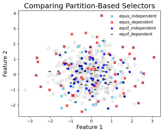
selector = GridPartition(nbins_axis=6, bin_method="equisized_independent")
selected_p1 = selector.select(X, size=size)
selector = GridPartition(nbins_axis=6, bin_method="equisized_dependent")
selected_p2 = selector.select(X, size=size)
selector = GridPartition(nbins_axis=6, bin_method="equifrequent_independent")
selected_p3 = selector.select(X, size=size)
selector = GridPartition(nbins_axis=6, bin_method="equifrequent_dependent")
selected_p4 = selector.select(X, size=size)
graph_data(
X,
indices=[selected_p1, selected_p2, selected_p3, selected_p4],
labels=[
# "Medoid",
"equis_independent",
"equis_dependent",
"equif_independent",
"equif_dependent",
],
title="Comparing Partition-Based Selectors",
xlabel="Feature 1",
ylabel="Feature 2",
fname="quick_start_compare_partition_methods",
)
Compute diversity of selected points#
div_measure = ["logdet", "wdud"]
set_labels = [
    # "Medoid",
    "equis_independent",
    "equis_dependent",
    "equif_independent",
    "equif_dependent",
]
set_indices = [selected_p1, selected_p2, selected_p3, selected_p4]
seleced_sets = zip(set_labels, set_indices)

# compute the diversity of the selected sets and render the results in a table
table_data = [[""] + div_measure]
for i in seleced_sets:
    # print([i[0]] + [compute_diversity(X_dist[i[1]], div_type=m) for m in div_measure])
    table_data.append([i[0]] + [compute_diversity(X_dist[i[1]], div_type=m) for m in div_measure])

render_table(table_data, caption="Diversity of Selected Sets")
Diversity of Selected Sets
| | logdet | wdud | |——————-|——————-|———————| | equis_independent | 90.84 | 0.072 | | equis_dependent | 90.513 | 0.063 | | equif_independent | 75.536 | 0.085 | | equif_dependent | 78.987 | 0.09 |
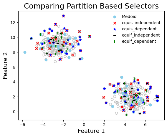
Comparing Multiple Selection Methods (Multiple Clusters)#
Each cluster is treated independently, and if possible, equal number of samples are selected from each cluster. However, if a cluster is underpopulated, then all points from that cluster are selected. This is to ensure that the selected subset is representative of the entire dataset.
# generate n_sample data in 2D feature space forming 3 clusters
X, labels = make_blobs(n_samples=500, n_features=2, centers=2, random_state=42)

# compute the (n_sample, n_sample) pairwise distance matrix
X_dist = pairwise_distances(X, metric="euclidean")

print("Shape of data   = ", X.shape)
print("Shape of labels = ", labels.shape)
print("Unique labels   = ", np.unique(labels))
size_0, size_1 = np.count_nonzero(labels == 0), np.count_nonzero(labels == 1)
print("Cluster sizes = ", size_0, size_1)
print("Shape of the distance array = ", X_dist.shape)
Shape of data   =  (500, 2)
Shape of labels =  (500,)
Unique labels   =  [0 1]
Cluster sizes =  250 250
Shape of the distance array =  (500, 500)
To select from multiple clusters provide the labels argument to the select method.
Check Documentation: Medoid | GridParition
# select data using grid partitioning methods
# -------------------------------------------
size = 50

selector = Medoid()
selected_medoid = selector.select(X, size=size, labels=labels)

selector = GridPartition(5, "equisized_independent")
selected_p1 = selector.select(X, size=size, labels=labels)

selector = GridPartition(5, "equisized_dependent")
selected_p2 = selector.select(X, size=size, labels=labels)

selector = GridPartition(5, "equifrequent_independent")
selected_p3 = selector.select(X, size=size, labels=labels)

selector = GridPartition(5, "equifrequent_dependent")
selected_p4 = selector.select(X, size=size, labels=labels)


graph_data(
    X,
    indices=[selected_medoid, selected_p1, selected_p2, selected_p3, selected_p4],
    labels=[
        "Medoid",
        "equis_independent",
        "equis_dependent",
        "equif_independent",
        "equif_dependent",
    ],
    title="Comparing Partition Based Selectors",
    xlabel="Feature 1",
    ylabel="Feature 2",
)
Compute the diversity of the selected data points#
div_measure = ["logdet", "wdud"]
set_labels = [
    # "Medoid",
    "equis_independent",
    "equis_dependent",
    "equif_independent",
    "equif_dependent",
]
set_indices = [selected_p1, selected_p2, selected_p3, selected_p4]
seleced_sets = zip(set_labels, set_indices)

# compute the diversity of the selected sets and render the results in a table
table_data = [[""] + div_measure]
for i in seleced_sets:
    # print([i[0]] + [compute_diversity(X_dist[i[1]], div_type=m) for m in div_measure])
    table_data.append([i[0]] + [compute_diversity(X_dist[i[1]], div_type=m) for m in div_measure])

render_table(table_data, caption="Diversity of Selected Sets")
Diversity of Selected Sets
| | logdet | wdud | |——————-|——————–|———————| | equis_independent | 118.897 | 0.081 | | equis_dependent | 117.838 | 0.079 | | equif_independent | 111.146 | 0.104 | | equif_dependent | 109.174 | 0.112 |